Compressed Filesystems á la Language Models

November 25, 2025 •

Every systems engineer at some point in their journey yearns to write a filesystem. This sounds daunting at first - and writing a battle-tested filesystem is hard - but the minimal surface area for a “working” FS is surprisingly small, simple, and in-distribution for coding agents.

In fact, one of my smoke tests for new coding models is seeing how good of a filesystem they can one-shot! At some point, I had quite a few filesystems lying around - and coding models were getting pretty good - which made me wonder if the models were intelligent enough to actually model the filesystem engine itself?

A filesystem is the perfect black-box API to model with wacky backends (see “Harder drives”), and besides the joy of training an LLM for fun - there were a few deeper truths about language models that I wanted to explore.

Training a filesystem #

So I set upon training a filesystem. Building on top of one of my throwaway FUSEs, a few rounds with Claude repurposed it to loopback against the host with added logging, two things I needed to generate reference fine-tuning data:

class LoggingLoopbackFS(LoggingMixIn, Operations):
    """
    A loopback FUSE filesystem that logs all operations for training data.
    
    This implementation delegates all filesystem operations to a real directory
    on the host filesystem, ensuring perfect semantic correctness while logging
    every operation for LLM training data.
    """

I then wrote a filesystem interaction simulator, which sampled various operations against a sandboxed LoggingLoopbackFS to generate diverse FUSE prompt/completion pairs. Concretely, I captured only the minimal set of operations needed for R/W-ish capability (no open, xattrs, fsync etc).

Alongside the FUSE operation, I captured the full filesystem state at every turn. I experimented with various formats, including an ASCII-art representation, but ultimately settled on XML since it enforces prompt boundaries clearly and had canonical parsers available.

With prompts including the FUSE operation + XML filesystem tree, the model learned two forms of completions:

Reads (<R>) requested the content / metadata as per the operation (getattr / readdir / read)
Writes (<W>) requested the model to output the full filesystem tree state, after modification (unlink / chmod / truncate / write)

Example prompt (read):

<R>
read('/usr14/log767.rs', size=4096, offset=0, fh=4) 
---
<filesystem>
  <directory path="/" name="/" mode="755" owner="root" group="root"
mtime="2025-01-01T00:00:00">
    <directory path="usr14" name="usr14" mode="755" owner="root" group="root"
mtime="2025-01-01T00:00:00">
      <file path="usr14/log767.rs" name="log767.rs" mode="644" owner="root"
group="root" mtime="2025-01-01T00:00:01" size="276">
        <body>fn main() {
    match process(7) {
        Ok(result) =&gt; println!("Result: {}", result),
        Err(e) =&gt; eprintln!("Error: {}", e),
    }
</body>
      </file>
      <file path="usr14/temp912.sh" name="temp912.sh" mode="644" owner="root"
group="root" mtime="2025-01-01T00:00:01" size="268">
        <body>#!/bin/bash 
         echo "temp912" || exit 1
       </body>
      </file>
    </directory>
  </directory>
</filesystem>

Completion:

fn main() {
    match process(7) {
        Ok(result) => println!("Result: {}", result),
        Err(e) => eprintln!("Error: {}", e),
    }
}

Fine-tuning #

Once I had clean, representative, and diverse filesystem simulation data, actually running SFT was pretty straightforward on Modal. Over a few iteration cycles spread across nibbles of spare time, I ended up with ~98% accuracy on a hold-out eval after 8 epochs of SFT on a N=15000 dataset with Qwen3-4b.

Most of my time here was spent cleaning generated data and ensuring we represented every FUSE operation sufficiently + generated enough “complex” trees to learn on.

At this point, I wrote … possibly the smallest filesystem I’ve seen… to give my model a spin in the real world. Every FUSE operation was a passthrough to the LLM, for example:

class LLMFuse(LoggingMixin, Operations):
    ...
    def chmod(self, path, mode):
        """Change file permissions."""
        response = self._query_llm_for_operation('chmod', path, mode=oct(mode))
        if not self._handle_llm_response(response):
            raise FuseOSError(ENOENT)
        return 0
    ...

Nice! I now had a mountable FUSE that was entirely “implemented” by a language model. As you can see below, I was able to ls around it, echo into files, and cat them back out.

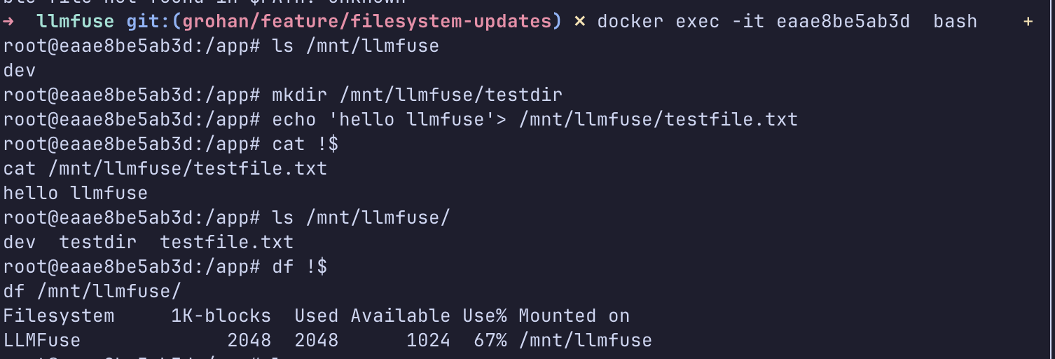Poking around a Docker container with a mounted LLMFuse.

Compressing the filesystem #

Perhaps the largest glaring inefficiency in this set up is the sheer verbosity of the XML-based representation. I was using many bytes to represent attributes and tree structure that could be encoded far more efficiently (~O(bits)) in a standard C struct.

However, as I was fine-tuning on the XML filesystem tree representation, I was baking in this very structure into the weights and probability distributions of my Qwen fork! If only there was a way to leverage this to compress state…

Two sides of the same coin #

As it turns out, compression and AI are intimately related. Using LLMs to lossily compress text is one of the most common applications, so it’s not entirely unintuitive. However, one researcher (Marcus Hutter) claimed back in 2006 that they are equivalent (and in fact bet $500K on this claim!).

Presciently, Hutter appears to be absolutely right. His enwik8 and enwik9’s benchmark datasets are, today, best compressed by a 169M parameter LLM (trained by none other than Fabrice Bellard in 2023).

That’s a bit perplexing on the first glance. Surely LLM compression isn’t reversible? What kind of voodoo magic was going on here?

Arithmetic coding #

The algorithm that enables reversible compression using LLMs is called “arithmetic coding” and it builds upon a 1948 result by Claude Shannon.

Researchers at DeepMind (including Hutter himself) have explained the math in detail, so I’ll direct the most inquisitive of you readers there, but for a simplified understanding of what’s going on, forget everything you might know about working with LLMs today. There’s no prompting involved!

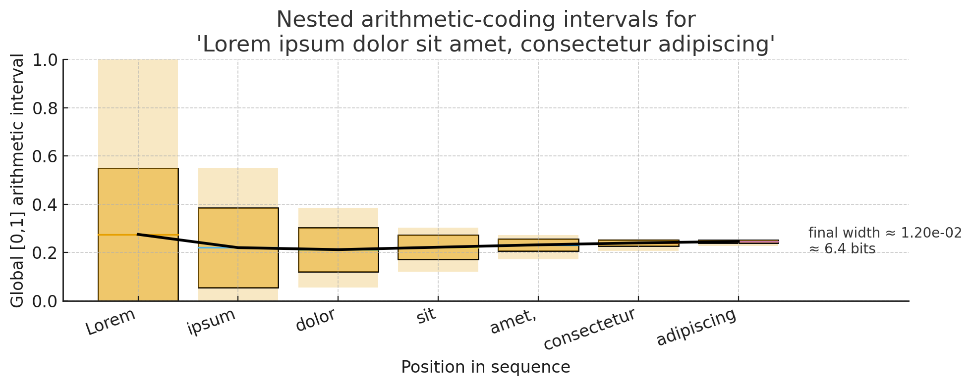
Let’s assume the following is true for some predictive model $M$

Lorem has first-word probability = 0.57.
Ipsum has second-word conditional probability = 0.67 (joint 0.38).
Dolor has a third word conditional probability = 0.5 (joint 0.19).

…

so on and so forth until you reach the end of the string you want to compress and you end up with some “final interval width” $P(m)$ on the real interval $[0,1]$ which represents your string.

Let’s suppose in our example this turns out to be 0.012. We can represent this decimal in roughly $- \log_{2}{P(m)} = 6.4$ bits, which is our final compression size.

There’s a few elegant things about this algorithm:

Any number within this interval is uniquely determined by tracing the arithmetic coding algorithm through the specific probabilistic model’s weights. “Decoding” is simply a retracing operation (see the line through the probability distributions above)
The inverse log relationship between predictive power $P(m)$ and compression pushes the burden of the “hard compression problem” to deep learning machinery which can encode high-dimensional text patterns within model weights, yielding far better compression ratios than deterministic algorithms.

Sounds cool! But how good really is this compression? On comparing arithmetic coding backed by Qwen3-4B against gzip for lipsum.txt, we already see pretty dramatic results:

Method	Size (bytes)	Compression Impact
Original (plain)	446	—
`gzip`	298	~33% smaller
`llmencode`	13	~97% smaller

(note: llmencode is my implementation of arithmetic coding)

22x better compression than gzip is pretty ridiculous! A caveat here is that lipsum.txt is heavily represented in training data, but 5-20x efficiency gains broadly hold for all text data that (looks like) it’s been on the internet.

Self-compression #

Now, back to our filesystem. The XML overhead we were worried about now can be “compressed away” by the fine-tuned model. Using the same toy filesystem from the Docker container demo above:

<filesystem>
  <directory path="/" name="/" mode="755" owner="root" group="root" mtime="2025-01-01T00:00:00">
    <directory path="testdir" name="testdir" mode="755" owner="root" group="root" mtime="2025-01-01T00:00:00" />
    <file path="testfile.txt" name="testfile.txt" mode="644" owner="root" group="root" mtime="2025-01-01T00:00:01" size="14">
      <body>hello llmfuse
</body>
    </file>
  </directory>
</filesystem>

Model	Original (bytes)	Compressed (bytes)	Ratio
Base Qwen3-4B	394	38	10.4x
Fine-tuned Qwen3-4B	394	21	18.8x

The fine-tuned model achieves 44.7% better compression on XML filesystem trees - the very format it was trained to predict. This is the “self-compression” effect: by baking the XML structure into the model weights during fine-tuning, the arithmetic coder can represent that structure in fewer bits.

Self-compression in filesystems isn’t a novel concept. For example, there exists the squashfs tool (created in 2002) to create R/O compressed filesystems. Squashfs compresses files, inodes, and directories together, not unlike what we’re doing here!

Under the hood, squashfs just wraps gzip/zstd/your favourite compression algorithm. So for plain-text data, squashfs compression stats pale in the face of llmfuse:

Method	Compressed Size	Notes
squashfs (gzip)	171 bytes	gzip-compressed file contents, inodes, directory tables
llmfuse (fine-tuned)	21 bytes	Arithmetic coded XML state

For the same filesystem tree (one directory, one 14-byte text file), llmfuse achieves ~8x better compression than squashfs (see methodology in appendix).

The difference comes down to llmencode being far better than gzip on text data + XML structure - especially when the model has been fine-tuned on exactly that structure.

Conclusion #

What started off as a little experiment mostly to get my hands dirty with training and inference evolved into a full blown nerd snipe and intellectual adventure. Thanks for making it this far!

I entirely recognize that this is a “toy” experiment under a very specific setup; with that said, the numbers above are pretty eye-popping, and the question I’ve been trying to answer as I write this up is: does this have any real-world potential?

Of course, in the short term, there’s a whole host of caveats: you need an LLM, likely a GPU, all your data is in the context window (which we know scales poorly), and this only works on text data.

Still, it’s intriguing to wonder whether the very engines that will likely dominate all “text generation” going forward can be used to compress their own data? Perhaps in a distant future, where running LLMs at the edge makes sense, or for specific kinds of workflows where data is read very infrequently.

Overall, I’m grateful to Peyton at Modal for the compute credits. Running a somewhat unconventional experiment like this wouldn’t have been possible without full control over the training and inference code, and extremely tedious without the simplicity of running ML infra on Modal! It’s truly awesome to be able to just modal deploy and get my own private inference endpoints, or just modal run to prototype some code on the cloud.

Appendix #

Source Code #

All of the source code for this experiment, particularly llmfuse and llmencode are open-sourced under MIT.

llmencode is abstracted into a CLI utility that you can run locally. Inference on 4B models is slow, but entirely possible on consumer hardware. I prototyped most of this code by running on a 2021 MacBook Pro, before productionizing on Modal.

A fun experiment / party trick to identify how “common” a certain string is in training data is to look at its llmencode compression ratio!

SquashFS comparison methodology #

The raw .sqsh file is 4096 bytes due to block alignment padding. To find the actual compressed size, I used xxd to inspect the binary and found the last non-zero byte at offset 266 (267 bytes total). Subtracting the fixed 96-byte superblock header gives us 171 bytes of actual gzip-compressed content - everything needed to reconstruct the filesystem.

Compression as a metric #

It’s equally interesting to think about compression as a metric. An angle I’d considered is doing some kind of RL on the arithmetic coded compression number itself.

Is that simply equivalent to the pre-training objective (due to the prediction-compression duality)? Or does the “sequence-level” objective add something more… interesting to the mix. Please reach out if you have thoughts!